Process Simulation
Process simulation allows you to simulate the execution of business processes to find out about cycle times, costs and resources. It can also be used to test the impact of changes between different variants of processes and then select the best variant for implementation. Process simulation thus helps you to determine and quantitatively evaluate the need for improvement. This makes simulation an important tool in process analysis and optimisation.
For which model types is process simulation enabled?
Process simulation is enabled for Business Process Diagrams.
Where can I configure the data the simulation is based on?
Unless otherwise stated, all attributes that need to be considered can be found in the Notebook chapter "Simulation data".
What Information do I need to get started?
To simulate a business process with meaningful results, you have to define at least the following simulation data:
The Execution time of all included Tasks.
The probability of alternative paths starting from an Exclusive gateway. It can be defined in the Transition condition attributes of the outgoing Sequence flows.
noteIn its simplest form, transition conditions are represented by floating point numbers
≥0 and≤1 (e.g. 0.7). The sum of the probabilities of all alternative paths starting from a gateway has to be 1.
How can I perform a cost analysis with personnel costs?
To perform a cost analysis with personnel costs, you have to determine the responsible roles and reference them in a business process:
For each Task, assign the responsible Roles in the Responsible for execution attribute (Notebook chapter "RACI").
At the Roles, enter the Hourly wages of the employees.
Enter the estimated non-personnel Costs of performing the Tasks.
How can process simulation help with capacity planning?
For capacity planning, you need to determine how often a process occurs:
- At the Start event, specify the Quantity (= number of occurrences) of this business process within the chosen Time period.
The attributes listed above are just a minimal set. In the following section, the attribute requirements for process simulation are examined more closely.
Process simulation is only available in the ADONIS NP Enterprise Edition. The availability of this feature also depends on the licence and the application library. All examples and descriptions in this chapter refer exclusively to the ADONIS BPMS Application Library.
If you are looking for a more lightweight solution than the process simulation, the process stepper provides a quick overview of specific process paths.
Prepare Model for Simulation
Before you can simulate the execution of a business process, certain requirements need to be fulfilled. These requirements fall into two categories:
Requirements for the model structure
Requirements for the attributes
Read on to learn more about these requirements.
Start Events
The Start Event indicates where a particular process will start.

Model Structure Requirements
- Every Business Process Diagram must contain exactly one Start Event object, which symbolizes the beginning of the process.
Attribute Requirements
- To show how often a process takes place, you need to fill in the attributes Quantity and Time period. If the Quantity attribute is empty, simulation will run with the default value "100". The default value for Time period is "Per Year".
Example
Tasks
A Task is an activity within a process flow. Tasks can have assigned costs and times. If they are performed by people, it is also possible to take work costs into account (see Role to learn more).

Model Structure Requirements
- Tasks should be part of a process flow.
Attribute Requirements
To specify how long it takes to perform a Task, use the Execution time attribute. Waiting time allows you to show time before work begins, while Resting time and Transport time show delays after a Task was executed.
To state that carrying out a Task generates costs, use the Costs attribute.
You can also assign one or more Roles to a Task in the Responsible for execution attribute (Notebook chapter "Organisation"). If you select two or more Roles, it is assumed all of them are needed for carrying out the Task.
Example
Subprocesses
A Subprocess is an activity that encapsulates a process. It allows you to show that certain parts of a process are described in detail in the linked sub model.

Simulation does not support inline Subprocesses (including "Ad-Hoc").
Model Structure Requirements
- To reference a Business Process Diagram from a Subprocess, use the Referenced subprocess attribute (Notebook chapter "General information"). The linked sub model will also be simulated. If there is no linked sub model, simulation data can be defined directly at the Subprocess.
Attribute Requirements
Ideally, all attributes are calculated based on the analysis of the sub model, so you do not need to adapt any attributes apart from the Referenced subprocess attribute.
If there is no linked sub model, or if the relevant information should be taken directly from the Subprocess, select the Use aggregated subprocess values check box. In this case, the relevant simulation data has to be defined directly at the Subprocess (see Tasks to learn more about the required attributes).
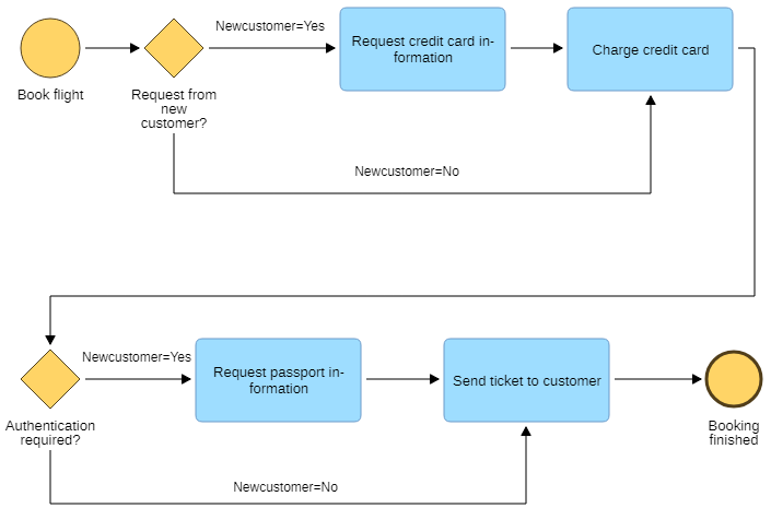
Exclusive Gateways and Sequence Flows
An Exclusive Gateway is used to create alternative paths within a process flow where only one of the paths can be taken.

Model Structure Requirements
- Model splitting paths using Exclusive Gateways, not Conditional Sequence Flows.
Attribute Requirements
To define the probability of alternative paths starting from an Exclusive gateway, adapt the Transition condition attributes of the outgoing Sequence flows.
In its simplest form, transition conditions are represented by floating point numbers
≥0 and≤1 (e.g. 0.7).
The sum of probabilities for outgoing paths has to be 1. If no probabilities are defined, the simulation is performed under the assumption that all alternative paths occur with the same frequency (e.g. 50/50 for 2 outgoing paths). If transition conditions are defined for some, but not all outgoing paths, the simulation mechanism will calculate the remaining probability (what is missing to reach 100%) and distribute it evenly across all paths without a defined probability.
Example
Advanced Methods of Defining Transition Conditions
The method described above of representing transition conditions by floating point numbers can be considered as a discrete distribution.
When a process contains loops, you can use floating point numbers to assign different probabilities for consecutive executions of the loops. You can find out more about this in the section Limit Number of Loops.
In addition to floating point numbers, you can also use variables in discrete distributions. These can be used at different points in the process to define transition conditions. You can find out more about this in the section Decide Process Path Based on Dependent Probabilities.
In addition to the discrete distribution ADONIS NP also supports different types of continuous distributions: These are the normal distribution, the exponential distribution and the uniform distribution. To learn more about these probability distributions that can be used to specify the probability of alternative paths during process simulation, see Probability Distributions.
Non-Exclusive Gateways
Non-exclusive Gateways allow you to show that multiple paths are executed simultaneously.

Model Structure Requirements
- Fork and join parallel paths using Non-exclusive Gateways which are defined as Parallel gateways (attribute Gateway type in the Notebook chapter "General information").
The simulation mechanism only supports Parallel Gateways for the simulation of simultaneously
running tasks. Inclusive Gateways
![]() are treated like Exclusive
Gateways by the simulation.
are treated like Exclusive
Gateways by the simulation.
Intermediate Events
Intermediate Events are events that take place during a process.

In BPMN 2.0, there are two basic categories of Intermediate Events: those belonging to a process flow and those attached to the boundaries of activities.
Intermediate Events (sequence flow) are not evaluated by the simulation. To document delay in your process caused e.g. by waiting for a message from an external pool, use the Waiting time attribute in the subsequent Task.
Intermediate events (boundary) allow you to show that certain events can take place during execution of a Task. They can be interrupting or non-interrupting (attribute Type in the Notebook chapter "Event type") You can define:
How probable it is that the event occurs while the Task is being executed (attribute Probability of occurrence).
If the Task is interrupted, what percentage of the Task is complete, that is, what fraction of costs and times should be added to the simulation results (attribute Rate of activity completion at event occurrence).
Model Structure Requirements
- Intermediate events (boundary) need to be attached to a Task (attribute Attached to in the Notebook chapter "General information").
Attribute Requirements
- Adapt the Probability of occurrence and Rate of activity completion at event occurrence
attributes. Both parameters are defined by floating point numbers
≥0 and≤1 (e.g. 0.7). The default values for both attributes are set to "0.5".
End Events
End Events indicate where a process path will end.

Model Structure Requirements
- Model an End Event for each path to allow a more in-depth analysis of the process results after a simulation run.
Roles
Roles define responsibility for Tasks. They are used for calculating personnel costs and capacities.

Attribute Requirements
- Adapt the Hourly wages attribute to allow calculating the personnel costs of your process.
Example
Run Simulation
In order to simulate one specific model:
Open the model in the graphical editor.
Click the More button
 in the
menu bar of the open model, point to Process analysis
in the
menu bar of the open model, point to Process analysis
 , and then click Simulation.
Define the simulation parameters:
In the Number of calculation cycles box, type the number of times you want ADONIS NP to simulate the model.
In the Working days per year box, type the number of working days per year.
In the Working hours per day box, type the number of working hours per day.
noteThe higher the number in the Number of calculation cycles box, the more accurately the probabilities of process paths are calculated, but the duration of the simulation will increase accordingly.
Working days per year and Working hours per day are used to calculate required resources and aggregate time values.
Working hours per day are expressed in decimal hours (for example, 7 hours and 30 minutes = 7.5).
For more information on these parameters, click the buttons
 next to the boxes.
Click Start.
Checks are run to find out if the model is ready for simulation. The results of the checks are shown in the "Validation" widget at the right side of the program window.
If no errors are found, the simulation results will be generated. When the calculation has finished, the simulation results are displayed.
Compare As-Is and To-Be Models
In addition to simulating one specific process, you can directly compare different variants of models. This allows you to test changes and work out where improvements are needed. To start a simulation with multiple models:
Select two or more models in the Model Catalogue.
Right-click the selection, and then click Simulation.
Advanced (Different Business Hours and Working Hours)
Select this option if the business hours of your company and the individual working hours are different. You must define the following simulation parameters:
In the Working days per year (employee) box, type the average number of days in a year in which an employee is performing work.
In the Working hours per day box, type the average number of hours per day in which an employee is performing work.
In the Business days per year (company) box, type the number of days in a year in which business is conducted and processes are executed.
In the Business hours per day (company) box, type the number of hours per day in which business is conducted and processes are executed.
Example
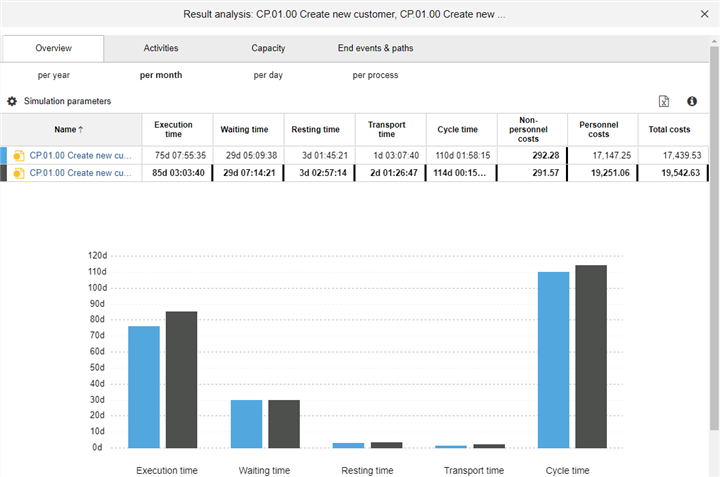
Interpret the Simulation Results
Once the simulation is complete, you can examine the results. By default, an overview of the results is displayed. Additional tabs provide more detailed information.
The following four tabs are available for evaluating and analysing the results:
An overview of the simulation results.
Drill-down to see how costs are accumulated at each activity. Supports Activity-based Costing (ABC).
How many full-time employees need to be allocated to this process? Full Time Equivalent (FTE) calculation tool.
Find out which paths lead to which process results and how often they occur. Enables detailed analysis of process paths in terms of time and cost (critical paths, number of paths, expensive paths, etc.). Also offers the possibility to display the paths graphically in the model.
Types of Results Data
Each simulation provides the following results (spread over the four simulation tabs):
Execution time
Specifies the average time necessary for completing activities.
Waiting time
Specifies how much time is needed on average as waiting time prior to execution of activities or while activities are interrupted.
Resting time
Specifies the average time in which activities "rest" after execution.
Transport time
Specifies the average time necessary for transport between the execution of different activities.
Cycle time
Specifies how much time is needed on average from the start of a process to its end (in other words, the response times to customers for customer-related processes).
Non-personnel costs
Specifies the costs of executing activities (not related to the wages of process performers).
Personnel costs
Personnel costs are calculated by multiplying the Execution time of a Task by the Hourly wage of the assigned Role.
Example
Total costs
For the total costs, non-personnel costs and personnel costs are added together.
# executions
The (average) number of executions of activities.
Capacity
Calculated number of full-time employees with the given role needed to perform activities within a given time period. This number assumes that an employee is performing only tasks in the simulated process, without any overheads (depending on working hours per day).
Example
Probability
The probability of an End Event occurring in percent (%).
Show Average Results per Hour, Month, Year or Process
In all simulation tabs, you can view results per process or for all processes over a time period:
To display the average results per process, click the per process button.
To display results for all processes, click either the per year, per month or per day buttons.
For the calculation of the results for all processes, the following factors all have an impact:
the Quantity and the Time period defined in the Process Start
the Working days per year and Working hours per day selected when starting the simulation
the observation period selected in the result table (per year, per month or per day)
Example
Overview
This tab provides an overview of the simulation results. The simulation results are displayed as follows:
Average results per process or for all processes over a time period are displayed in a table. The result table contains one line for every simulated process. The following information is displayed:
Average process times
Average process costs
Additionally, key metrics are represented graphically below the table:
If you only simulate one specific process, this data is represented in a pie chart.
If you simulate multiple models, key metrics are represented by a bar chart. This is especially useful for comparing As-Is and To-Be models, as you can see at a glance which variant performs better.
Change Simulation Parameters
To change the simulation parameters and re-run the simulation:
- Click the Change simulation parameters button.
This enables you to view results based on different values.
Activities
The Activities tab provides detailed information about process steps. You can drill-down to see how costs are accumulated at each Task and which activities are often performed.
In the result table, the activities are listed. They are grouped by model, and sorted according to the order in the model. Each model in the simulation is listed with all activities, including sub models which are referenced from a Subprocess. The following information is displayed:
Responsible roles
Number of executions
Times
Costs
Capacity
Capacity
The Capacity tab provides detailed information for personnel planning. You can find out how many full-time employees with the given role are needed to perform a process within a given time period.
In the result table, the Roles are listed. They are grouped by model, and sorted alphabetically. Each model in the simulation is listed with all Roles, including sub models which are referenced from a Subprocess. The following information is displayed:
Capacity
Times
Costs
Group by Roles
To group the result by Roles:
- Point to the header of the Name column, click the button
 , and then click group by this
field.
, and then click group by this
field.
In this view, you can find out how much in total each Role is needed.
End Events & Paths
The End events & paths tab allows you to analyse End Events to see how often process results occur. This will enable you to answer questions such as:
How many job applications per year do I accept and how many do I reject?
How many credit requests per month do I accept and how many do I reject?
How many times does a product not meet quality requirements?
In the result table, the End Events are listed. They are grouped by model, and sorted alphabetically. Each model in the simulation is listed with all End Events (sub models are not included). The following information is displayed:
Number of executions
Probability
Times
Costs
Path Analysis and Visualisation
To analyse alternative paths within a process flow in more detail:
In the result table, click any End Event to open the "Simulation Paths" widget at the right side of the program window.
From the lists at the top of the widget, select the following:
the Process
the End Event
the Time Period you want to analyse
Select Time Period: Per Process vs. Single Path ResultsTo display the average results per process, select per process.
To display the exact results for a path run, select single path results.
All paths leading to the selected process end are displayed. For each path, you can see the probability of it occurring, and the times and costs associated with it. Use the sorting options to find out which path is the most critical, longest, shortest, most likely, most expensive, etc.
Visualise Path
To visualise a path in a model:
- Click the link to the path in the result.
The model is opened in the graphical editor. The objects that match this path are highlighted on the drawing area. Numbers indicate how often a step was executed (useful for loops).
Alternatively, you can show the path as a list:
- Click the Show path flow button
 next to the link.
Sort Table Contents
By default, the paths are sorted alphabetically. To change this sorting, proceed as follows:
Click the header of a column to sort the table by its content (ascending).
Click on the column header again to reverse the sorting order from ascending to descending (and vice versa).
Select Columns
To select which columns to display:
The button
is activated in the
header of any column by mouseover. Click this button to open a drop-down menu.Point to Columns, and then choose the desired columns.
Alternatively, you can hide and show entire categories of results:
- To hide categories, click the Hide times and Hide costs buttons. These buttons are toggles. Click them again to show the categories again.
Group Paths
To group paths:
- Click the Group paths button.
All unique paths are placed in the Unique Paths group. Separate groups (Group 1, Group 2, etc.) contain paths that only differ in the number of consecutive executions of a loop, but are otherwise identical.
End Event What-If Analysis
The What-If Analysis allows calculating times and costs assuming that an End Event occurs a certain number of times. This will enable you to answer questions such as:
- This year I'm selling 700 contracts. Next year it will be 1400. What does this mean in terms of time and costs?
To run a What-If Analysis:
In the result table, click any End Event to open the "Simulation Paths" widget at the right side of the program window.
From the What if the End Event list, select the End Event you want to analyse.
In the had been reached ... times? box, type the number of times this End Event should occur.
Click Calculate.
The results of the What-If Analysis are displayed. In the result table, the paths are listed. They are grouped by End Event, and sorted alphabetically. For each path, the following information is displayed:
Number of executions
Probability
Times
Costs
Below, in the capacity table, you can see how many full-time employees with the given role are needed to perform the process assuming the End Event occurs a certain number of times.
At the bottom, in the cost driver table, you can see the total times and costs to perform the process assuming that the End Event occurs a certain number of times (first row) or once (second row).
Advanced Methods
This section explains advanced methods for defining transition conditions.
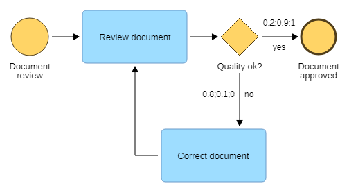
Limit Number of Loops
When a process contains loops, you can assign different probabilities for consecutive executions of the loops. This enables you to specify that the chance that a Task will be completed successfully increases (or decreases) with each run.
Attribute Requirements
To define the probability of alternative paths starting from an Exclusive gateway, adapt the Transition condition attributes of the outgoing Sequence flows.
Transition conditions are represented by floating point numbers
≥0 and≤1 (e.g. 0.7). The sum of the probabilities of all alternative paths starting from a gateway has to be 1.For loops, assign more than one probability, so that the value changes after consecutive executions. Separate the values with a ";". The simulation runs through the loop the first time with the first values, then with the second values and so on.
Example
Decide Process Path Based on Dependent Probabilities
Recurring transition values can be defined via variables. To determine paths in a process, the same variable value will always be used after branchings. This way, it is possible to define depending probabilities.
Attribute Requirements
To define a variable, select a Sequence flow in the process. Click the icon
 to add a new row in the
attribute Variables. Specify the name (first column), distribution type (second column) and
the distribution parameters (third column).
to add a new row in the
attribute Variables. Specify the name (first column), distribution type (second column) and
the distribution parameters (third column).To use the variable for alternative paths starting from an Exclusive gateway, adapt the Transition condition attributes of the outgoing Sequence flows. Specify the variable name, an operator and a constant.
Defining all variables in a Sequence flow at the beginning of the process makes it easier to find them when a change is necessary.
For more information on these parameters, click the buttons
![]() next to the attributes.
next to the attributes.
Example
Probability Distributions
In this section, we are going to take a closer look at the probability distributions that can be used to specify the probability of alternative paths during process simulation. The following probability distributions are possible:
Discrete Distribution
In discrete distributions, each variable assumes a fixed (discrete) value.
Continuous Distribution
Normal distribution, exponential distribution and uniform distribution. In continuous distributions, the focus is on intervals (a range of values which the variable can assume).
Probability distributions are defined via variables.
Attribute Requirements
To define a variable, select a Sequence flow in the process. Open the Notebook and select the chapter "Simulation data". Click the icon
 to add a new row in the
attribute Variables. Specify the name (first column), distribution type (second column) and
the distribution parameters (third column).
to add a new row in the
attribute Variables. Specify the name (first column), distribution type (second column) and
the distribution parameters (third column).To use the variable for alternative paths starting from an Exclusive gateway, adapt the Transition condition attributes of the outgoing Sequence flows. Specify the variable name, an operator and a constant. Two or more variables can be logically joined using the logical operators AND and OR.
Discrete Distribution
A discrete distribution has a finite number of values.

Notation in ADONIS NP
In order to define a discrete distribution, enter two or more symbols with their corresponding probabilities. The sum of the probabilities must always equal 1.
For example, the Variable "VariableX", "Discrete", "Normal case (0.4); Exception1 (0.3); Exception2 (0.3)" is assigned the value "Normal case" with a probability of 40%, and the values "Exception1" and "Exception2" with a probability of 30% each.
Example
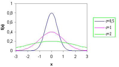
Normal Distribution
The normal distribution (or Gaussian distribution) is the most important type of continuous probability distribution.
Notation in ADONIS NP
In order to define a normal distribution, two parameters are needed: the expected value and the standard deviation.
For example, the Variable "VariableX", "Normal", "0\@2" has a normal distribution with an expected value of 0 and a standard deviation of 2.
Example


Exponential Distribution
The exponential distribution is a continuous probability distribution over a set of positive real numbers. It is often used to model the time elapsed between events.
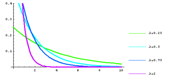
Notation in ADONIS NP
In order to define an exponential distribution, enter the value of the exponential distribution, which is 1 divided by the expected value (1/E).
For example, the Variable "VariableX", "Exponential", "0.5" has an exponential distribution with an expected value of 2.
Example


Uniform Distribution
The uniform distribution describes a probability distribution in which the same probability of being true exists for all values between an upper and a lower limit.

Notation in ADONIS NP
In order to define a uniform distribution, enter the boundaries for the uniform distribution where the first number is the lower boundary and the second number is the upper boundary.
For example, the Variable "VariableX", "Uniform", "20\@100" has a uniform distribution between 20 and 100.
Example


Export Simulation Results
To export the simulation results as an Excel file (XLSX format):
- Click the Export results button
 .
.
In the Excel spreadsheet, the results from the currently selected tab are shown.